Hierachical Logistic Regression
Let’s set some setting for this Jupyter Notebook.
In [3]:
%matplotlib inline
from warnings import filterwarnings
filterwarnings("ignore")
import os
os.environ['MKL_THREADING_LAYER'] = 'GNU'
os.environ['THEANO_FLAGS'] = 'device=cpu'

import numpy as np
import pandas as pd
import pymc3 as pm
import seaborn as sns
import matplotlib.pyplot as plt
np.random.seed(12345)
rc = {'xtick.labelsize': 20, 'ytick.labelsize': 20, 'axes.labelsize': 20, 'font.size': 20,
      'legend.fontsize': 12.0, 'axes.titlesize': 10, "figure.figsize": [12, 6]}
sns.set(rc = rc)
from IPython.core.interactiveshell import InteractiveShell
InteractiveShell.ast_node_interactivity = "all"
Now, let’s import the HierarchicalLogisticRegression model from the
pymc-learn package.
In [4]:
import pmlearn
from pmlearn.linear_model import HierarchicalLogisticRegression
print('Running on pymc-learn v{}'.format(pmlearn.__version__))
Running on pymc-learn v0.0.1.rc0
Step 1: Prepare the data
Generate synthetic data.
In [5]:
num_pred = 2
num_samples = 700000
num_categories = 2
In [6]:
alphas = 5 * np.random.randn(num_categories) + 5 # mu_alpha = sigma_alpha = 5
betas = 10 * np.random.randn(num_categories, num_pred) + 10 # mu_beta = sigma_beta = 10
In [7]:
alphas
Out[7]:
array([ 3.9764617 , 7.39471669])
In [8]:
betas
Out[8]:
array([[  4.80561285,   4.44269696],
       [ 29.65780573,  23.93405833]])
In [9]:
def numpy_invlogit(x):
    return 1 / (1 + np.exp(-x))
In [10]:
x_a = np.random.randn(num_samples, num_pred)
y_a = np.random.binomial(1, numpy_invlogit(alphas[0] + np.sum(betas[0] * x_a, 1)))
x_b = np.random.randn(num_samples, num_pred)
y_b = np.random.binomial(1, numpy_invlogit(alphas[1] + np.sum(betas[1] * x_b, 1)))

X = np.concatenate([x_a, x_b])
y = np.concatenate([y_a, y_b])
cats = np.concatenate([
    np.zeros(num_samples, dtype=np.int),
    np.ones(num_samples, dtype=np.int)
])
In [11]:
from sklearn.model_selection import train_test_split
X_train, X_test, y_train, y_test, cats_train, cats_test = train_test_split(X, y, cats, test_size=0.3)
Step 2: Instantiate a model
In [12]:
model = HierarchicalLogisticRegression()
Step 3: Perform Inference
In [13]:
model.fit(X_train, y_train, cats_train, minibatch_size=2000, inference_args={'n': 60000})
Average Loss = 246.46: 100%|██████████| 60000/60000 [02:19<00:00, 429.21it/s]
Finished [100%]: Average Loss = 246.56
Out[13]:
HierarchicalLogisticRegression()
Step 4: Diagnose convergence
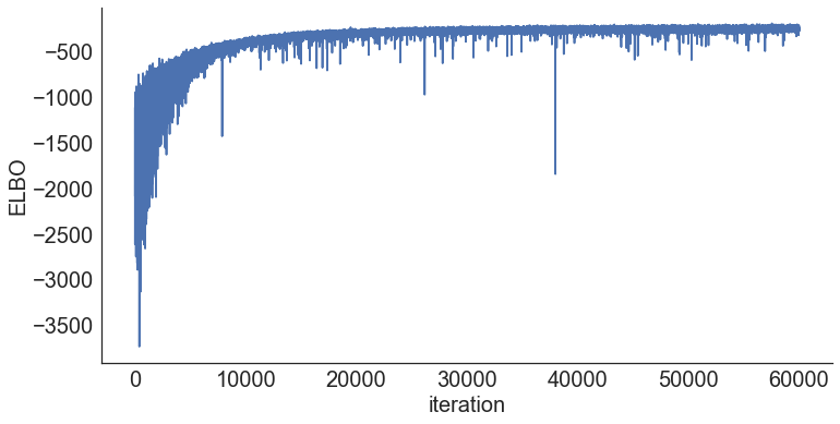
In [14]:
model.plot_elbo()
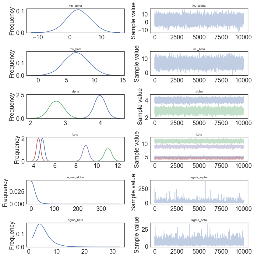
In [15]:
pm.traceplot(model.trace);
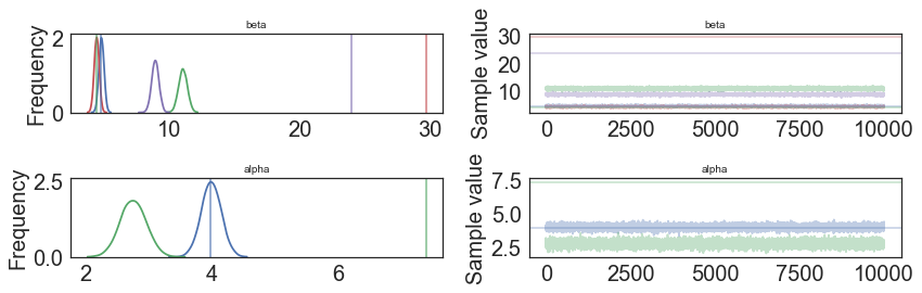
In [16]:
pm.traceplot(model.trace, lines = {"beta": betas,
                                 "alpha": alphas},
             varnames=["beta", "alpha"]);
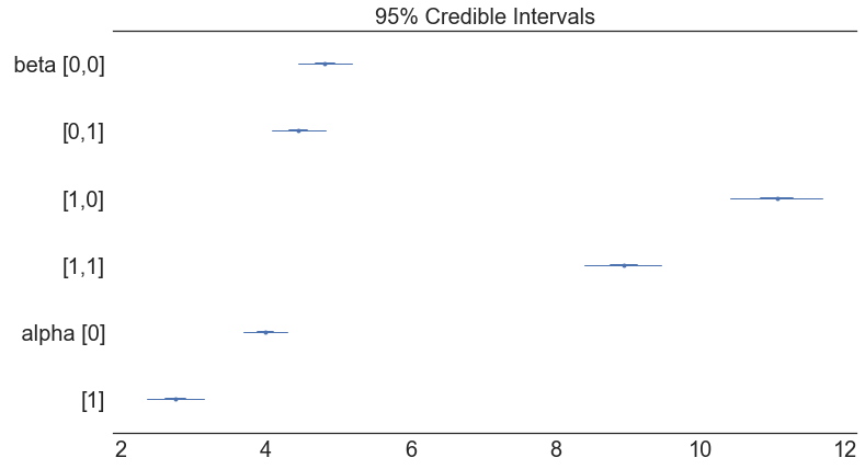
In [17]:
pm.forestplot(model.trace, varnames=["beta", "alpha"]);
Step 5: Critize the model
In [18]:
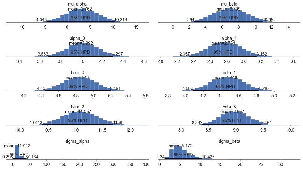
pm.summary(model.trace)
Out[18]:
| mean | sd | mc_error | hpd_2.5 | hpd_97.5 | |
|---|---|---|---|---|---|
| mu_alpha | 2.762447 | 3.702337 | 0.035507 | -4.345352 | 10.213894 |
| mu_beta | 6.799099 | 2.119254 | 0.020894 | 2.640162 | 10.953644 |
| alpha__0 | 3.992272 | 0.154989 | 0.001559 | 3.683080 | 4.296882 |
| alpha__1 | 2.753978 | 0.203159 | 0.002084 | 2.356660 | 3.152206 |
| beta__0_0 | 4.817129 | 0.190077 | 0.001997 | 4.449666 | 5.191381 |
| beta__0_1 | 4.447704 | 0.186797 | 0.002043 | 4.086421 | 4.817914 |
| beta__1_0 | 11.057359 | 0.327623 | 0.002926 | 10.413378 | 11.689952 |
| beta__1_1 | 8.937158 | 0.271224 | 0.002630 | 8.392272 | 9.461213 |
| sigma_alpha | 11.912198 | 15.283716 | 0.165522 | 0.294809 | 37.133923 |
| sigma_beta | 5.171519 | 2.691029 | 0.028385 | 1.340010 | 10.425355 |
In [19]:
pm.plot_posterior(model.trace, figsize = [14, 8]);
In [20]:
# collect the results into a pandas dataframe to display
# "mp" stands for marginal posterior
pd.DataFrame({"Parameter": ["beta", "alpha"],
               "Parameter-Learned (Mean Value)": [model.trace["beta"].mean(axis=0),
                                model.trace["alpha"].mean(axis=0)],
               "True value": [betas, alphas]})
Out[20]:
| Parameter | Parameter-Learned (Mean Value) | True value | |
|---|---|---|---|
| 0 | beta | [[4.81712892701, 4.44770360874], [11.057358919... | [[4.80561284943, 4.44269695653], [29.657805725... |
| 1 | alpha | [3.99227159692, 2.75397848498] | [3.97646170258, 7.39471669029] |
Step 6: Use the model for prediction
In [21]:
y_probs = model.predict_proba(X_test, cats_test)
100%|██████████| 2000/2000 [02:07<00:00, 15.50it/s]
In [22]:
y_predicted = model.predict(X_test, cats_test)
100%|██████████| 2000/2000 [02:12<00:00, 15.66it/s]
In [23]:
model.score(X_test, y_test, cats_test)
100%|██████████| 2000/2000 [02:10<00:00, 15.18it/s]
Out[23]:
0.95806190476190478
In [24]:
model.save('pickle_jar/hlogistic_model')
Use already trained model for prediction
In [25]:
model_new = HierarchicalLogisticRegression()
In [26]:
model_new.load('pickle_jar/hlogistic_model')
In [27]:
model_new.score(X_test, y_test, cats_test)
100%|██████████| 2000/2000 [01:25<00:00, 23.49it/s]
Out[27]:
0.95800952380952376
MCMC
In [ ]:
model2 = HierarchicalLogisticRegression()
model2.fit(X_train, y_train, cats_train, inference_type='nuts')
In [ ]:
pm.traceplot(model2.trace, lines = {"beta": betas,
                                 "alpha": alphas},
             varnames=["beta", "alpha"]);
In [ ]:
pm.gelman_rubin(model2.trace)
In [ ]:
pm.energyplot(model2.trace);
In [ ]:
pm.summary(model2.trace)
In [ ]:
pm.plot_posterior(model2.trace, figsize = [14, 8]);
In [ ]:
y_predict2 = model2.predict(X_test)
In [ ]:
model2.score(X_test, y_test)
In [ ]:
model2.save('pickle_jar/hlogistic_model2')
model2_new = LogisticRegression()
model2_new.load('pickle_jar/hlogistic_model2')
model2_new.score(X_test, y_test, cats_test)