Logistic Regression¶

Let’s set some setting for this Jupyter Notebook.

In [1]:

%matplotlib inline
from warnings import filterwarnings
filterwarnings("ignore")
import os
os.environ['MKL_THREADING_LAYER'] = 'GNU'
os.environ['THEANO_FLAGS'] = 'device=cpu'

import numpy as np
import pandas as pd
import pymc3 as pm
import seaborn as sns
import matplotlib.pyplot as plt
np.random.seed(12345)
rc = {'xtick.labelsize': 20, 'ytick.labelsize': 20, 'axes.labelsize': 20, 'font.size': 20,
      'legend.fontsize': 12.0, 'axes.titlesize': 10, "figure.figsize": [12, 6]}
sns.set(rc = rc)
from IPython.core.interactiveshell import InteractiveShell
InteractiveShell.ast_node_interactivity = "all"

Now, let’s import the LogisticRegression model from the pymc-learn package.

In [2]:

import pmlearn
from pmlearn.linear_model import LogisticRegression
print('Running on pymc-learn v{}'.format(pmlearn.__version__))

Running on pymc-learn v0.0.1.rc0

Step 1: Prepare the data¶

Generate synthetic data.

In [3]:

num_pred = 2
num_samples = 700000
num_categories = 2

In [4]:

alphas = 5 * np.random.randn(num_categories) + 5 # mu_alpha = sigma_alpha = 5
betas = 10 * np.random.randn(num_categories, num_pred) + 10 # mu_beta = sigma_beta = 10

In [5]:

alphas

Out[5]:

array([ 3.9764617 ,  7.39471669])

In [6]:

betas

Out[6]:

array([[  4.80561285,   4.44269696],
       [ 29.65780573,  23.93405833]])

In [7]:

def numpy_invlogit(x):
    return 1 / (1 + np.exp(-x))

In [8]:

x_a = np.random.randn(num_samples, num_pred)
y_a = np.random.binomial(1, numpy_invlogit(alphas[0] + np.sum(betas[0] * x_a, 1)))
x_b = np.random.randn(num_samples, num_pred)
y_b = np.random.binomial(1, numpy_invlogit(alphas[1] + np.sum(betas[1] * x_b, 1)))

X = np.concatenate([x_a, x_b])
y = np.concatenate([y_a, y_b])
cats = np.concatenate([
    np.zeros(num_samples, dtype=np.int),
    np.ones(num_samples, dtype=np.int)
])

In [9]:

from sklearn.model_selection import train_test_split
X_train, X_test, y_train, y_test, cats_train, cats_test = train_test_split(X, y, cats, test_size=0.3)

Step 2: Instantiate a model¶

In [10]:

model = LogisticRegression()

Step 3: Perform Inference¶

In [11]:

model.fit(X_train, y_train, cats_train, minibatch_size=2000, inference_args={'n': 60000})

Average Loss = 249.45: 100%|██████████| 60000/60000 [01:13<00:00, 814.48it/s]
Finished [100%]: Average Loss = 249.5

Out[11]:

LogisticRegression()

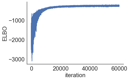
Step 4: Diagnose convergence¶

In [12]:

model.plot_elbo()

../_images/notebooks_LogisticRegression_18_0.png

In [13]:

pm.traceplot(model.trace);

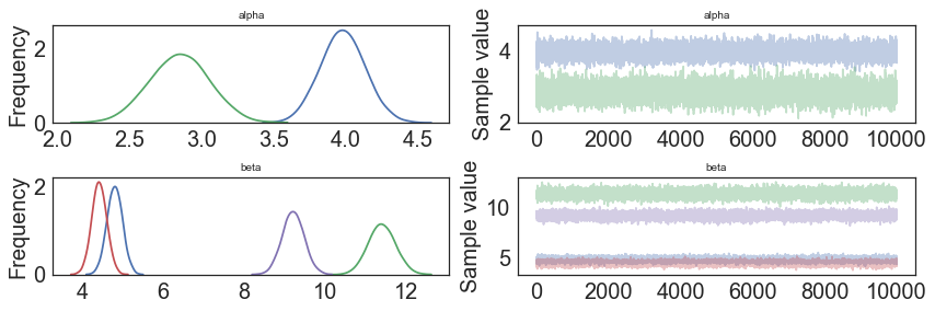
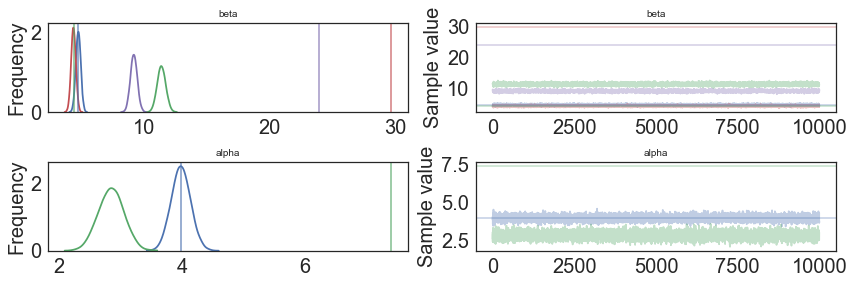
../_images/notebooks_LogisticRegression_19_0.png

In [14]:

pm.traceplot(model.trace, lines = {"beta": betas,
                                 "alpha": alphas},
             varnames=["beta", "alpha"]);

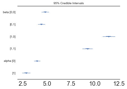
../_images/notebooks_LogisticRegression_20_0.png

In [15]:

pm.forestplot(model.trace, varnames=["beta", "alpha"]);

../_images/notebooks_LogisticRegression_21_0.png

Step 5: Critize the model¶

In [16]:

pm.summary(model.trace)

Out[16]:

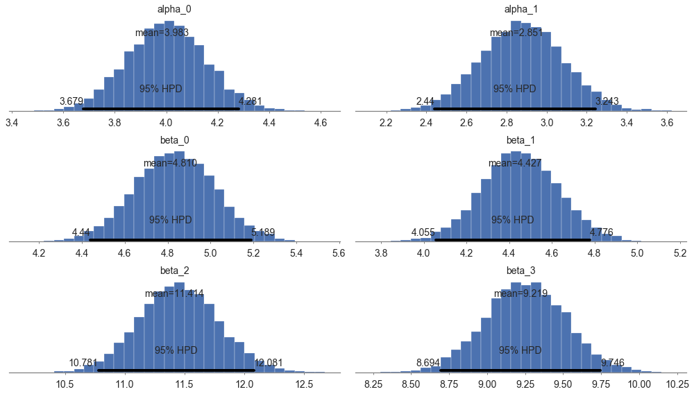
	mean	sd	mc_error	hpd_2.5	hpd_97.5
alpha__0	3.982634	0.153671	0.001556	3.678890	4.280575
alpha__1	2.850619	0.206359	0.001756	2.440148	3.242568
beta__0_0	4.809822	0.189382	0.001727	4.439762	5.188622
beta__0_1	4.427498	0.183183	0.001855	4.055033	4.776228
beta__1_0	11.413951	0.333251	0.003194	10.781074	12.081359
beta__1_1	9.218845	0.267730	0.002730	8.693964	9.745963

In [17]:

pm.plot_posterior(model.trace, figsize = [14, 8]);

../_images/notebooks_LogisticRegression_24_0.png

In [18]:

# collect the results into a pandas dataframe to display
# "mp" stands for marginal posterior
pd.DataFrame({"Parameter": ["beta", "alpha"],
               "Parameter-Learned (Mean Value)": [model.trace["beta"].mean(axis=0),
                                model.trace["alpha"].mean(axis=0)],
               "True value": [betas, alphas]})

Out[18]:

	Parameter	Parameter-Learned (Mean Value)	True value
0	beta	[[4.80982191646, 4.4274983607], [11.413950812,...	[[4.80561284943, 4.44269695653], [29.657805725...
1	alpha	[3.98263424275, 2.85061932727]	[3.97646170258, 7.39471669029]

Step 6: Use the model for prediction¶

In [19]:

y_probs = model.predict_proba(X_test, cats_test)

100%|██████████| 2000/2000 [01:24<00:00, 23.62it/s]

In [20]:

y_predicted = model.predict(X_test, cats_test)

100%|██████████| 2000/2000 [01:21<00:00, 24.65it/s]

In [21]:

model.score(X_test, y_test, cats_test)

100%|██████████| 2000/2000 [01:23<00:00, 23.97it/s]

Out[21]:

0.9580642857142857

In [22]:

model.save('pickle_jar/logistic_model')

Use already trained model for prediction¶

In [23]:

model_new = LogisticRegression()

In [25]:

model_new.load('pickle_jar/logistic_model')

In [26]:

model_new.score(X_test, y_test, cats_test)

100%|██████████| 2000/2000 [01:23<00:00, 24.01it/s]

Out[26]:

0.9581952380952381

MCMC¶

In [ ]:

model2 = LogisticRegression()
model2.fit(X_train, y_train, cats_train, inference_type='nuts')

In [ ]:

pm.traceplot(model2.trace, lines = {"beta": betas,
                                 "alpha": alphas},
             varnames=["beta", "alpha"]);

In [ ]:

pm.gelman_rubin(model2.trace)

In [ ]:

pm.energyplot(model2.trace);

In [ ]:

pm.summary(model2.trace)

In [ ]:

pm.plot_posterior(model2.trace, figsize = [14, 8]);

In [ ]:

y_predict2 = model2.predict(X_test)

In [ ]:

model2.score(X_test, y_test)

In [ ]:

model2.save('pickle_jar/logistic_model2')
model2_new = LogisticRegression()
model2_new.load('pickle_jar/logistic_model2')
model2_new.score(X_test, y_test, cats_test)